QG Omega equation
07 April 2022 by MiniUFO, Yuan Zhao, and Lei Liu
[TOC]
1. Introduction
Quasi-geostrophic omega (\(\omega\)) equation is a classical diagnostic model valid at synoptic- to large-scales away from equator and the poles. In atmospheric context, \(\omega=dp/dt\) means the vertical motion (\(Pa\) \(s^{-1}\)) in pressure- (\(p\)-) coordinates. In oceanic context, it recovers the vertical motion (\(m\) \(s^{-1}\)) in the depth- (\(z\)-) coordinates as \(w\) .
The QG-omega equation is derived from the QG approximation. Also, it is a 3D equation that involves derivatives along three spatial dimentions (\(x,y,z\)). Therefore, it is somewhat complicated than the 2D inverse problems. Traditionally, the forcing function on the rhs of the equation contains two terms. As a result, this equation is useful in diagnosting the contributions to the vertical motion from the two terms, which respresent different physical processes.
2. Theory
2.1 Derivation of the QG omega equation
Here the derivation of the QG omega equation is briefly reviewed. The start point, in the atmospheric context, is the primitive equation set in spherical-pressure coordinates:
where \(\partial x=a\cos\phi\partial \lambda\) and \(\partial y=a\partial\phi\) are the short-hands. The QG approximations are:
define the geostrophic flow as \(\mathbf{v_g}=f^{-1}\hat\nabla\Phi\), where \(\hat\nabla\equiv(-\partial/\partial y, \partial/\partial x)\) is the 90° anti-clockwise rotation of \(\nabla\equiv(\partial/\partial x, \partial/\partial y)\);
introduce geostrophic vorticity \(\zeta_g=\hat\nabla\cdot\mathbf{v_g}=\hat\nabla^2\Phi=\nabla^2\Phi\);
decompose the full flow into geostrophic and ageostrophic components \(\mathbf{v}=\mathbf{v_g}+\mathbf{v_a}\) and assume \(\mathbf{v_g}\gg\mathbf{v_a}\);
momentum advection is accomplished by \(\mathbf{v_g}\) i.e., neglect the vertical advection by \(\omega\) in the momentum equation [the vertical heat advection in Eq. (5) is retained];
neglect the metrics terms in spherical coordinates.
Then we have the QG equation set as:
The derivation of the QG omega equation is much clear if 1) the momentum equation is first combined into the vorticity equation, with Eq. (9) to remove the divergence of ageostrophic wind, 2) apply the \(\hat\nabla^2\) to both sides of Eq. (8):
Notice that \(\hat\nabla\cdot\mathbf{F}\) is the curl of external forcing. Then taking \(\partial/\partial t\) on both sides of Eq. (12), and using Eqs. (11) and (13) to eliminate the tendency tems, one obtains the QG omega equation:
where \(S=-\frac{R\pi}{p}\frac{\partial \theta}{\partial p}\) is the static stability or buoyancy frequency.
2.1 Traditional form
The traditional form involves further assumptions of adiabatic (\(\dot\theta=0\)) and invisid (\(\mathbf{F}=0\)) dynamics, \(f\)-plane approximation (\(f=f_0\)), and that the static stability \(S\) does not vary horizontally. Upon this, the traditional form of QG omega equation is:
For oceanic context, \(\theta\) is replaced by buoyancy \(b\equiv-\rho g/\rho_0\) (note that \(S=\partial b/\partial z\)), and the QG-equation is somewhat simplified:
2.2 Q-vector form
Hoskins et al. (1978) provided an alternative form of the QG omega equation through manipulating the two forcing terms on the rhs of Eq. (16). The resulting equation is known as the Q-vector form of the QG omega equation (without diabatic and frictional forcings):
where the Q-vector is defined in atmospheric context as:
and in oceanic context as:
The Q-vector form has several advantages over the traditional form:
Forcing function (Q-vector) is evaluated on a single vertical level [see Eq. (18)]. Traditional form requires information at 3 levels to take vertical derivatives. Note that one can also express Q-vector in terms of geopotential \(\Phi\) alone and the QG-omega can be determined by 3D distribution of \(\Phi\) completely [Eq. (18’)]. But it is not well-defined at the equator because \(f\) tends to be zero.
Forcing function is Galilean invariant.
In the traditional form, adevction between temperature and vorticity usually cancel each other. In Q-vector form, no cancellation problem between forcing terms.
Q-vectors can be plotted on geopotential height and temperature maps to obtain representation of forcing for vertical motion, ageostrophic circulation, and frontogenesis.
3. Examples
Here we will demonstrate how to use xinvert python package to calculate QG vertical motion using gridded data. The inversion requires a simple calculation of the forcing function, which is not included in xinvert. However, with the help of xarray, this is relatively simple. ### 3.1 Global atmospheric example The first example is the inversion using global atmospheric reanalysis data from JRA (a single timestep). First, loading the data into xarray.Dataset:
[1]:
import sys
sys.path.append('../../../')
import xarray as xr
import numpy as np
from xinvert import FiniteDiff

Rd = 287.04
Cp = 1004.88
omega = 7.292e-5

############ load JRA global reanalysis sample data ###########
ds = xr.open_dataset('../../../Data/atmos3D.nc', decode_times=False)
ds['LEV'] = ds['LEV'] * 100

################## calculate basic variables ##################
fd = FiniteDiff({'X':'lon', 'Y':'lat', 'Z':'LEV'},
                BCs={'X':('periodic','periodic'),
                     'Y':('reflect','reflect'),
                     'Z':('extend','extend')}, fill=0, coords='lat-lon')

############# zonal running smooth of polar grids ###############
def smooth(v, gridpoint=13, lat=80):
    rolled = v.pad({'lon':(gridpoint,gridpoint)},mode='wrap')\
              .rolling(lon=gridpoint, center=True, min_periods=1).mean()\
              .isel(lon=slice(gridpoint, -gridpoint))
    return xr.where(np.abs(v-v+v.lat)>lat, rolled, v)

# smooth out zonal grid-scale noise
T   = smooth(ds.T, lat=85)
U   = smooth(ds.U, lat=85)
V   = smooth(ds.V, lat=85)
W   = smooth(ds.Omega, lat=85)
H   = smooth(ds.hgt, lat=85)

p   = ds.LEV
Psfc= ds.psfc

f    = 2*omega*np.sin(np.deg2rad(ds.lat)) # Coriolis parameter
th   = T * (100000 / p)**(Rd/Cp)   # potential temperature
TH   = th.mean(['lat','lon']) # domain-mean
vor  = fd.curl(U,V).load() # vorticity to approx. geostrophic vorticity
_, tmp = xr.broadcast(vor, vor.mean('lon'))
vor[:,0,:] = tmp[:,0,:]
vor[:,-1,:] = tmp[:,-1,:]
dTHdp= TH.differentiate('LEV')
RPiP = (Rd * T / p / TH)
S    = - RPiP * dTHdp              # static stability parameter

################ traditional form of forcings Eq. (15) ################
grdthx, grdthy = fd.grad(th , ['X', 'Y'])
grdvrx, grdvry = fd.grad(vor, ['X', 'Y'])

F1 = fd.Laplacian((U * grdthx + V * grdthy) * RPiP)
F2 = ((U * grdvrx + V * grdvry) * f).differentiate('LEV')

FAll = (F1 + F2)
FAll = smooth(xr.where(np.isinf(FAll), np.nan, FAll), lat=85)

################# Q-vector form of forcings Eq. (18) #################
ux, uy = fd.grad(U, ['X', 'Y'])
vx, vy = fd.grad(V, ['X', 'Y'])

Qx = - RPiP * (ux * grdthx + vx * grdthy)
Qy = - RPiP * (uy * grdthx + vy * grdthy)

FQvec = -2 * fd.divg((Qx, Qy), dims=['X', 'Y'])
FQvec = smooth(xr.where(np.isinf(FQvec), np.nan, FQvec), lat=85)
We also prepare to use the surface \(\omega\) as the lower boundary condition for the inversion:
[2]:
#%% prepare lower boundary for inversion
p3D = T-T+p # broadcast

FAll2  =  FAll.where(p<=Psfc)
FQvec2 = FQvec.where(p<=Psfc)

WBC = xr.where(p3D<=Psfc, 0, W).load()
Now inverting for omegas. Note that the whole inversion requires two variables: the forcing function \(F\) and static stability parameter \(S\) (which only varies in the vertical).
[3]:
### inverting ###
from xinvert import invert_omega

iParams = {
    'BCs'      : ['fixed', 'fixed', 'periodic'],
    'mxLoop'   : 5000,
    'tolerance': 1e-16,
}

mParams = {'N2': S}

WQG    = invert_omega(FAll  , dims=['LEV', 'lat', 'lon'], iParams=iParams, mParams=mParams)
WQvec  = invert_omega(FQvec , dims=['LEV', 'lat', 'lon'], iParams=iParams, mParams=mParams)
WQG2   = invert_omega(FAll2 , dims=['LEV', 'lat', 'lon'], iParams=iParams, mParams=mParams, icbc=WBC)
WQvec2 = invert_omega(FQvec2, dims=['LEV', 'lat', 'lon'], iParams=iParams, mParams=mParams, icbc=WBC)
{} loops 3601 and tolerance is 0.000000e+00
{} loops 2975 and tolerance is 0.000000e+00
{} loops 5000 and tolerance is 8.074381e-11
{} loops 5000 and tolerance is 6.564631e-11
Now we can plot the results. First take a look at the pattern on an upper level.
[4]:
# plot horizontal plane
import proplot as pplt

fontsize = 11
z = 25 # 375 hPa
array = [[1,1,2,2], [3,3,4,4], [0,5,5,0]]

fig, axes = pplt.subplots(array, figsize=(7, 5.7), proj=pplt.Proj('cyl', lon_0=180))

ax = axes[0]
m=ax.contourf(WQG[z], levels=np.linspace(-0.1, 0.1, 21), cmap='RdBu_r', extend='both')
ax.set_title('inverted QG omega (traditional)')
ax = axes[1]
m=ax.contourf(WQG2[z], levels=np.linspace(-0.1, 0.1, 21), cmap='RdBu_r', extend='both')
ax.set_title('inverted QG omega (trad. with topo)')
ax = axes[2]
m=ax.contourf(WQvec[z], levels=np.linspace(-0.1, 0.1, 21), cmap='RdBu_r', extend='both')
ax.set_title('inverted QG omega (Q-vector)')
ax = axes[3]
m=ax.contourf(WQvec2[z], levels=np.linspace(-0.1, 0.1, 21), cmap='RdBu_r', extend='both')
ax.set_title('inverted QG omega (Q-vec. with topo)')
ax = axes[4]
m=ax.contourf(W[z], levels=np.linspace(-0.1, 0.1, 21), cmap='RdBu_r', extend='both')
ax.set_title('observed omega')
ax.colorbar(m, loc='r', cols=(1,2), length=0.85, label='')

axes.format(abc='(a)', coast=True, grid=False, labels=False)
C:\ProgramData\anaconda3\lib\site-packages\cartopy\mpl\geoaxes.py:406: UserWarning: The `map_projection` keyword argument is deprecated, use `projection` to instantiate a GeoAxes instead.
  warnings.warn("The `map_projection` keyword argument is "
C:\ProgramData\anaconda3\lib\site-packages\cartopy\mpl\geoaxes.py:406: UserWarning: The `map_projection` keyword argument is deprecated, use `projection` to instantiate a GeoAxes instead.
  warnings.warn("The `map_projection` keyword argument is "
C:\ProgramData\anaconda3\lib\site-packages\cartopy\mpl\geoaxes.py:406: UserWarning: The `map_projection` keyword argument is deprecated, use `projection` to instantiate a GeoAxes instead.
  warnings.warn("The `map_projection` keyword argument is "
C:\ProgramData\anaconda3\lib\site-packages\cartopy\mpl\geoaxes.py:406: UserWarning: The `map_projection` keyword argument is deprecated, use `projection` to instantiate a GeoAxes instead.
  warnings.warn("The `map_projection` keyword argument is "
C:\ProgramData\anaconda3\lib\site-packages\cartopy\mpl\geoaxes.py:406: UserWarning: The `map_projection` keyword argument is deprecated, use `projection` to instantiate a GeoAxes instead.
  warnings.warn("The `map_projection` keyword argument is "

Plot a cross section to demonstrate the difference between different lower boundary conditions.
[7]:
import proplot as pplt

x = 80
fontsize = 13
array = [[1,1,2,2], [3,3,4,4], [0,5,5,0]]

fig, axes = pplt.subplots(array, figsize=(7, 5.7), sharex=3, sharey=3)

ax = axes[0]
m=ax.pcolormesh(WQG[:, :, x].where(p3D[:, :, x]<=Psfc[:,x]), levels=np.linspace(-0.1, 0.1, 21), cmap='RdBu_r')
ax.set_title('inverted QG omega (traditional)')
ax = axes[1]
m=ax.pcolormesh(WQG2[:, :, x].where(p3D[:, :, x]<=Psfc[:,x]), levels=np.linspace(-0.1, 0.1, 21), cmap='RdBu_r')
ax.set_title('inverted QG omega (trad. with topo)')
ax = axes[2]
m=ax.pcolormesh(WQvec[:, :, x].where(p3D[:, :, x]<=Psfc[:,x]), levels=np.linspace(-0.1, 0.1, 21), cmap='RdBu_r')
ax.set_title('inverted QG omega (Q-vector)')
ax = axes[3]
m=ax.pcolormesh(WQvec2[:, :, x].where(p3D[:, :, x]<=Psfc[:,x]), levels=np.linspace(-0.1, 0.1, 21), cmap='RdBu_r')
ax.set_title('inverted QG omega (Q-vec. with topo)')
ax = axes[4]
m=ax.pcolormesh(W[:, :, x].where(p3D[:, :, x]<=Psfc[:,x]), levels=np.linspace(-0.1, 0.1, 21), cmap='RdBu_r')
ax.set_title('observed omega')
ax.colorbar(m, loc='r', length=1, label='')

axes.format(abc='(a)', ylim=[100000, 10000], xlim=[-90,90], ylabel='', xlabel='')
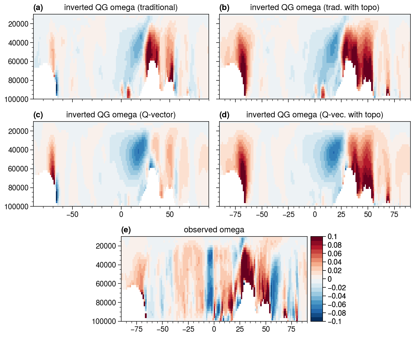
It is clear that the solutions forced by traditional and Q-vector forms are similar in general. Difference may be due to the finite difference schemes. With lower boundary values close to that of observed one, the inverted omega will match the observed one when approaching the lower boundary. Maybe we should loop from the top to the bottom, where the upper boundary condition is set to \(\omega=0\). Also, in the tropics, as the forcing term vanished there, the vertical motion is relatively weak. One needs to add diabatic forcing to the forcing function to produce more similar pattern in the tropics.
3.2 Oceanic example
We use the OFES reanalysis data over Kuroshio extension region to demonstrate the application in oceanic context. This case is well demonstrated in Liu et al. (2021).
[1]:
#%% load converted netcdf from Lei Liu
import sys
sys.path.append('../../../')
import numpy as np
import xarray as xr
import pooch

# We are working with a regional OFES data (~3GB)
fname = pooch.retrieve(
    url="doi:10.6084/m9.figshare.23712933.v2/data.nc",
    known_hash="md5:c9018bed7bf55898e5319ba44d9dc213",
)

ds = xr.open_dataset(fname, chunks={'lev':6}).astype('f4')

# dset = ds.sel({'lon':slice(143.1, 150.9), 'lat':slice(31.1, 38.9)})
ds['lev'] = -ds['lev'] # Reverse the z-coord. positive direction
                       # This is important for taking vertical derivatives.
C:\ProgramData\anaconda3\lib\site-packages\paramiko\transport.py:219: CryptographyDeprecationWarning: Blowfish has been deprecated
  "class": algorithms.Blowfish,
Then we calculate the QG forcings according to Eqs. (16) and (19).
[2]:
#%% calculate QG forcings
from xinvert import FiniteDiff

fd = FiniteDiff({'X':'lon', 'Y':'lat', 'Z':'LEV'},
                BCs={'X':('extend','extend'),
                     'Y':('extend','extend'),
                     'Z':('extend','extend')}, fill=0, coords='lat-lon')

u = ds.u / 100 # change unit from cm/s to m/s
v = ds.v / 100 # change unit from cm/s to m/s
w = ds.w / 100 # change unit from cm/s to m/s

b  = ds.rho * (-9.81/1023)
f  = 2 * 7.292e-5 * np.sin(np.deg2rad(ds.lat))
N2 = b.mean(['lat','lon']).load().differentiate('lev').load()

########## traditional form of forcings ##########
bx, by = fd.grad(b, ['X', 'Y'])
zx, zy = fd.grad(fd.curl(u, v), ['X', 'Y'])

adv_b = u*bx + v*by
adv_z = u*zx + v*zy

Ftrad = fd.Laplacian(-adv_b, ['X', 'Y']) + adv_z.load().differentiate('lev')*f
Ftrad = (xr.where(np.isfinite(Ftrad), Ftrad, np.nan)).load()

############ Q-vector form of forcings ############
ux, uy = fd.grad(u, ['X', 'Y'])
vx, vy = fd.grad(v, ['X', 'Y'])

Qx = ux*bx + vx*by
Qy = uy*bx + vy*by

divQ  = -2 * fd.divg((Qx, Qy), ['X', 'Y'])
FQvec = xr.where(np.isfinite(divQ), divQ, np.nan).load()

#%% maskout topography
WBC1 = xr.where(np.isnan(Ftrad), 0, w)
WBC2 = xr.where(np.isnan(FQvec), 0, w)
Then we can perform inversion similarly:
[3]:
import time
from xinvert import invert_omega

iParams = {
    'BCs'      : ['fixed', 'fixed', 'extend'],
    'mxLoop'   : 500,
    'tolerance': 1e-9,
}

mParams = {'N2': N2}

start = time.time()
W1 = invert_omega(Ftrad, dims=['lev', 'lat', 'lon'], iParams=iParams, mParams=mParams).load()
W2 = invert_omega(FQvec, dims=['lev', 'lat', 'lon'], iParams=iParams, mParams=mParams).load()
W1t= invert_omega(Ftrad, dims=['lev', 'lat', 'lon'], iParams=iParams, mParams=mParams, icbc=WBC1).load()
W2t= invert_omega(FQvec, dims=['lev', 'lat', 'lon'], iParams=iParams, mParams=mParams, icbc=WBC2).load()
elapsed = time.time() - start
print('time used: ', elapsed)
{} loops  500 and tolerance is 3.134166e-04
{} loops  500 and tolerance is 3.249085e-04
{} loops  500 and tolerance is 4.052368e-04
{} loops  500 and tolerance is 4.071324e-04
time used:  2920.084809064865
Results can be plotted as:
[4]:
#%% plot and compare
import proplot as pplt

fontsize = 13
array = [[1,1,2,2], [3,3,4,4], [0,5,5,0]]
z = 10 # choose subsurface to show

fig, axes = pplt.subplots(array, figsize=(8.6, 7.5), sharey=3, sharex=3)

ax = axes[0]
m=ax.pcolormesh(W1[z]*1e4, levels=np.linspace(-2, 2, 21), cmap='RdBu_r')
ax.set_title('inverted QG w (traditional)', fontsize=fontsize)

ax = axes[1]
m=ax.pcolormesh(W2[z]*1e4, levels=np.linspace(-2, 2, 21), cmap='RdBu_r')
ax.set_title('inverted QG w (Q-vector)', fontsize=fontsize)

ax = axes[2]
m=ax.pcolormesh(W1t[z]*1e4, levels=np.linspace(-2, 2, 21), cmap='RdBu_r')
ax.set_title('inverted QG w (traditional topo.)', fontsize=fontsize)
ax = axes[3]
m=ax.pcolormesh(W2t[z]*1e4, levels=np.linspace(-2, 2, 21), cmap='RdBu_r')
ax.set_title('inverted QG w (Q-vector topo.)', fontsize=fontsize)

ax = axes[4]
m=ax.pcolormesh(w[z]*1e4, levels=np.linspace(-2, 2, 21), cmap='RdBu_r')
ax.set_title('observed w', fontsize=fontsize)
fig.colorbar(m, loc='r', label='', rows=(1,3))

axes.format(abc='(a)', xlabel='', ylabel='')
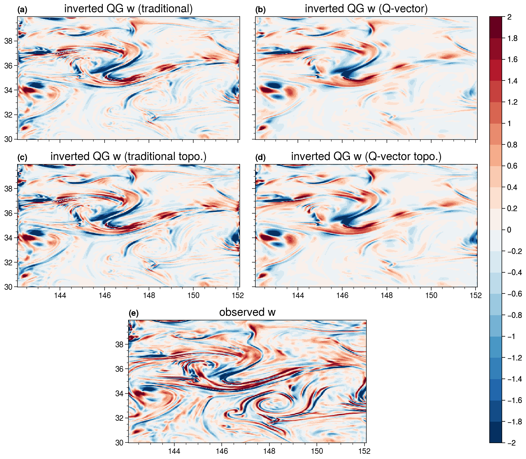
It is clear that the adiabatic QG forcings reproduce much of the vertical motion pattern. One may also need diabatic and frictional forcings to make it better.
References
Hoskins, B. J., I. Draghici, and H. C. Davies, 1978: A new look at the ω-equation. Q. J. R. Meteorol. Soc., 104, 31-38.
Liu, Lei,, H. Xue, and H. Sasaki, 2021: Diagnosing Subsurface Vertical Velocities from High-Resolution Sea Surface Fields. J. Phys. Oceanogr., 51, 1353–1373.