Reference state for shallow-water model
10 May 2023 by MiniUFO
[TOC]
1. Introduction
It is well known that 2D inviscid adiabatic shallow-water flow on the spherical earth is governed by:
Here \(\mathbf{\hat u}=(-v, u)\) is the anti-clockwise rotation of horizontal velocity vector \(\mathbf u\), \(\hat\nabla = (-\partial_y, \partial_x)\) is the horizontal curl operator, and \(q=(\hat\nabla\cdot \mathbf u+f)/h\) is the potential vorticity (PV). It is of great importance and interests to get a steady-state solution \(S_R=(h_R, u_R, v_R)\) of the above nonlinear equation set so that it satisfies:
That is, when the state of the fluid is in \(S_R\), nothing would change in the absence of forcing and dissipation. One of such steady-state solution is \(u_R=0\), \(v_R=0\), and \(h_R=constant\), which is a trivil motionless state with a flat surface (also known as Lorenz’s reference state or resting reference state). Here we are going to obtained another nontrivil \(S_R\) (nonresting reference state).
2. Theory
There are infinite solutions that satisfy Eqs. (3-4). To reduce the degree of freedom, we impose a constraint that \(S_R\) is symmetric along \(x\). This means that any derivative along \(x\) is 0 and \(S_R\) only varies with \(y\). Then Eq. (3) becomes:
The zonal symmetric constraint has eliminate \(v_R\), leaving a gradient-wind balance as Eq. (6).
It is well-known that the shallow-water Eqs. (1-2) conserve potential vorticity (PV) \(q=(\zeta+f)/h\), which is \(dq/dt=0\). As a result, any functions of PV is conserved. Two of these functions, total mass \(M\) and circulation \(C\) enclosed by PV contours, should also conserve:
Here \(Q\) is a set of PV contour values, \(M(Q)\) is the total mass enclosed by a contour \(Q\), and \(C(Q)\) is the circulation around \(Q\).
2.1 A balanced equation in terms of \(C\)
The conservation of mass indicates:
Here \(2\pi r\) is the length of latitude circle at \(\phi\). The zonal symmetry of \(S_R\) ensures the third equality in Eq. (9), as well as \(C=2\pi r(u_R+\Omega r)\). As a result, we have:
and a modified gradient-wind balance of Eq. (6):
Finally, with the identity \(Q\partial M/\partial y=\partial C/\partial y\), we have:
This is a 2nd-order elliptical equation about \(C\). Although it is nonlinear, it can be linearized about \(C_0=2\pi r(\overline u+\Omega r)\) as:
Here \(C_0\) is the Eulerian zonal mean circulation, which is treated as a known or a first guess during iteration. One could first invert Eq. (13) for \(C\), and then put the inverted \(C\) as \(C_0\) for a second inversion loop using Eq. (13). This is actually a nonlinear iteration loop for inverting Eq. (12). Since Eq. (12) is weakly nonlinear (i.e., \(C\) does not change significantly during iteration), inverting Eq. (12) is also possible by repeating this loop several times.
However, for a global domain, the presence of PV \(Q\) in the denominator can be problematic: PV could be zero near the equator. So inversion of Eq. (12) globally is generally NOT practical. We need another form of balanced equation in terms of \(M\).
2.2 A balanced equation in terms of \(\Delta M\)
Started with Eq. (11), if the initial guesses \(M_0\) and \(C_0\) are knowns, following Nakamura and Solomon (2011) and Thuburn and Lagneau (1999), we introduce a correction \(\Delta M = M - M_0\), and noting that:
then Eq. (11) is written as:
After some manipulations, it is cleaned up to:
This is the one-dimensional Screened Poisson eqaution about \(\Delta M\), as long as the coefficient of \(\Delta M\) is non-negative (generally \(Q_0\sin\phi\ge0\)). In this case, we can use xinvert to get the solutions.
3. Examples
Here we will demonstrate how to use xinvert python package to invert Eq. (14), and nonlinear loops for inverting Eq. (18), and hence the whole reference state. First we load a global dataset output from shallow-water model.
3.1 Inversion for reference state (steady state)
[1]:
import sys
sys.path.append('../../../')
import xarray as xr
import numpy as np

ds = xr.open_dataset('../../../Data/Barotropic2D.nc')
ds['time'] = np.arange(25)
print(ds)
<xarray.Dataset>
Dimensions:  (time: 25, lat: 241, lon: 480)
Coordinates:
  * time     (time) int32 0 1 2 3 4 5 6 7 8 9 ... 15 16 17 18 19 20 21 22 23 24
  * lat      (lat) float32 -90.0 -89.25 -88.5 -87.75 ... 87.75 88.5 89.25 90.0
  * lon      (lon) float32 0.0 0.75 1.5 2.25 3.0 ... 357.0 357.8 358.5 359.2
Data variables:
    u        (time, lat, lon) float32 ...
    v        (time, lat, lon) float32 ...
    h        (time, lat, lon) float32 ...
    zeta     (time, lat, lon) float32 ...
    uref     (time, lat) float32 ...
    href     (time, lat) float32 ...
    Mref     (time, lat) float32 ...
    Cref     (time, lat) float32 ...
    Qref     (time, lat) float32 ...
Attributes:
    comment:  U component of wind
    storage:  99
    title:    ERAInterim
    undef:    -999000000.0
    pdef:     None
Following Thuburn and Lagneau (1999), we first obtain the tabulated relations \(M(Q)\) and \(C(Q)\) using `xcontour <https://github.com/miniufo/xcontour>`__, where \(Q\) is a uniform set of PV contours from minimum to maximum values at each timestep. Then we use initial guess of mass as \(M_0=M_{\max}(1+sin\phi)/2\), and get \(Q_0\) and \(C_0\) through interpolating
the tabulated \(M(Q)\) and \(C(Q)\). With \(M_0\), \(Q_0\) and \(C_0\), one can solve for \(\Delta M\) (and hence \(M\)).
[3]:
try:  # if one has xcontour package installed
    from xcontour import Contour2D, add_latlon_metrics
    import xgcm
    print('calculate using xcontour and xgcm')

    # # add metrics for xgcm
    dset, grid = add_latlon_metrics(ds)

    N  = 201             # increase the contour number may get non-monotonic A(q) relation
    increase = True      # Y-index increases with latitude
    lt = True            # northward of PV contours (larger than) is inside the contour
                         # change this should not change the result of Keff, but may alter
                         # the values at boundaries
    dtype  = np.float32  # use float32 to save memory
    undef  = -999000000. # for maskout topography if present

    f  = 2 * 7.292e-5 * np.sin(np.deg2rad(ds.lat))
    PV = (ds.zeta / ds.h).rename('PV')

    # initialize a Contour2D analysis class using PV as the tracer
    analysis = Contour2D(grid, PV, dims={'X':'lon','Y':'lat'}, dimEq={'Y':'lat'},
                         increase=increase, lt=lt)

    # get Q, M(Q), C(Q)
    ctr  = analysis.cal_contours(N).rename('ctr')
    Mass = analysis.cal_integral_within_contours_hist(ctr, integrand=ds.h).rename('Mass')
    Circ = analysis.cal_integral_within_contours_hist(ctr, integrand=ds.zeta).rename('Circ') * -1.0

    # ensure both poles have zero circulation
    Circ = xr.where(Circ.contour==N-1, 0, Circ).transpose().rename('Circ')

except ImportError:
    print('load from a pre-calculated nc file')
    ds_ctr = xr.open_dataset('../../../Data/contour.nc')

    ctr = ds_ctr.PV
    Mass = ds_ctr.Mass
    Circ = ds_ctr.Circ

def getQandC(M):
    # get Qref and Cref given Mref, using linear interpolation and tabulated M(Q), C(Q)
    Q = xr.apply_ufunc(np.interp, M, Mass, ctr,
                       dask='parallelized',
                       input_core_dims=[['lat'], ['contour'], ['contour']],
                       vectorize=True,
                       output_core_dims=[['lat']])
    # ensure the north-pole consistency
    Q = xr.where(Q.lat==90, ctr.max('contour'), Q).transpose()
    C = xr.apply_ufunc(np.interp, Q, ctr, Circ,
                       dask='parallelized',
                       input_core_dims=[['lat'], ['contour'], ['contour']],
                       vectorize=True,
                       output_core_dims=[['lat']])
    return Q, C
load from a pre-calculated nc file
Now we do the inversion. But notice that we need to update \(M\), \(Q\), and \(C\) several times as it is a weakly nonlinear iteration. According to Thuburn and Lagneau (1999), three nonlinear loops would be OK. Here we use five loops.
[4]:
from xinvert import invert_RefStateSWM

iParams = {
    'BCs'      : ['fixed'],
    'mxLoop'   : 5000,
    'tolerance': 1e-18,
    'undef'    : np.nan,
    'debug'    : False,
    'printInfo': False}

# initial guess of Mref
Mref = Mass.max('contour') * (np.sin(np.deg2rad(ds.lat)) + 1.0) / 2.0

for i in range(5): # nonlinear loops for 5 times
    print(i)
    Qref, Cref = getQandC(Mref) # update Q and C
    mParams = {'M0':Mref, 'C0':Cref} # set as model parameters
    dM = invert_RefStateSWM(Qref, dims=['lat'], iParams=iParams, mParams=mParams)
    Mref = Mref + dM
0
1
2
3
4
Now we can get all the reference states \(Q_{R}\), \(u_{R}\), and \(h_{R}\) (note that \(v_{R}\equiv 0\)):
[5]:
r = 6371200. * np.cos(np.deg2rad(ds.lat))

uref = Cref / (2.0 * np.pi * r) - 7.292e-5 * r
href = Mref.differentiate('lat') / (2.0 * np.pi * r) / (6371200. * np.deg2rad(1.))
3.2 Comparison with the zonal-mean state
The zonal-mean state is usually used for eddy-mean flow decomposition. However, the zonal mean is only a diffused estimate of the reference state, because it does NOT conserve PV and mass. Also, zonal-mean state is NOT a steady state. Here we show their differences.
[6]:
import proplot as pplt

fontsize = 12

um = ds.u.mean('lon')
hm = ds.h.mean('lon')

fig, axes = pplt.subplots(nrows=3, ncols=2, figsize=(7, 7), sharex=3, sharey=3)

ax = axes[0, 0]
m = ax.contourf(um.T, levels=np.linspace(-45, 45, 19), cmap='seismic')
ax.set_title('um', fontsize=fontsize)

ax = axes[1, 0]
m = ax.contourf(uref.T, levels=np.linspace(-45, 45, 19), cmap='seismic')
ax.set_title('uref (python-code)', fontsize=fontsize)

ax = axes[2, 0]
m = ax.contourf(ds.uref.T, levels=np.linspace(-45, 45, 19), cmap='seismic')
ax.colorbar(m, loc='b')
ax.set_title('uref (Java-code)', fontsize=fontsize)

ax = axes[0, 1]
m = ax.contourf(hm.T, levels=np.linspace(400, 2300, 20), cmap='jet')
ax.set_title('hm', fontsize=fontsize)

ax = axes[1, 1]
m = ax.contourf(href.T, levels=np.linspace(400, 2300, 20), cmap='jet')
ax.set_title('href (python-code)', fontsize=fontsize)

ax = axes[2, 1]
m = ax.contourf(ds.href.T, levels=np.linspace(400, 2300, 20), cmap='jet')
ax.colorbar(m, loc='b')
ax.set_title('href (Java-code)', fontsize=fontsize)

axes.format(abc='(a)', xlabel='time (6hr)', ylabel='latitude')
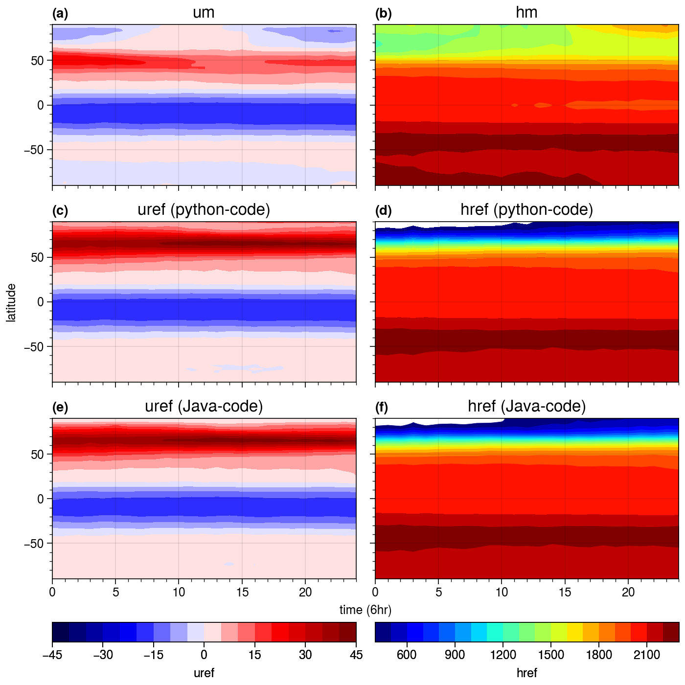
It is clear that the zonal-mean of jets is greatly weakened and its evolutionary timescale is shorter than the reference state. This indicates the reference state is a quasi-stationary solution. It only evolves in response to non-conservative processes (forcing and dissipation).
[7]:
import proplot as pplt
import cartopy.crs as ccrs
import warnings
warnings.filterwarnings('ignore')

PVp = (ds.zeta / ds.h).rename('PV') * 1e7 # in PV unit
PVm = PVp.mean('lon')
fontsize = 12

def plot_step(axes, idx, step):
    thres = 0.75
    levels = np.linspace(-5, 5, 21)
    m = axes[idx, 0].contour(PVp[step], cmap='jet', lw=1,
                   levels=[-0.2, 0, 0.2, 0.4, 0.6, 1, 1.4, 1.8, 2.4, 3, 4, 5, 7, 9])
    PVa = PVp-PVm
    PVa = PVa.where(np.abs(PVa)>=thres)
    m = axes[idx, 1].contourf(PVa[step], cmap='seismic', zorder=3, levels=levels, extend='both')
    m = axes[idx, 1].contour((PVp-PVp+PVm)[step], cmap='jet', lw=1, zorder=4,
                   levels=[-0.2, 0, 0.2, 0.4, 0.6, 1, 1.4, 1.8, 2.4, 3, 4, 5, 7, 9])
    PVa = PVp-Qref * 1e7
    PVa = PVa.where(np.abs(PVa)>=thres)
    m = axes[idx, 2].contourf(PVa[step], cmap='seismic', zorder=3, levels=levels, extend='both')
    m = axes[idx, 2].contour((PVp-PVp+Qref)[step]*1e7, cmap='jet', lw=1, zorder=4,
                   levels=[-0.2, 0, 0.2, 0.4, 0.6, 1, 1.4, 1.8, 2.4, 3, 4, 5, 7, 9])
    axes[idx, 0].set_title(f't = {step/4.0} day', fontsize=fontsize)
    axes[idx, 1].set_title(f't = {step/4.0} day', fontsize=fontsize)
    axes[idx, 2].set_title(f't = {step/4.0} day', fontsize=fontsize)
    return m

fig, axes = pplt.subplots(nrows=3, ncols=3, figsize=(7, 7),
                          proj=ccrs.NearsidePerspective(central_latitude=60, central_longitude=165))

plot_step(axes, 0,  0)
plot_step(axes, 1, 10)
plot_step(axes, 2, 24)

axes.format(abc='(a)', land=True, coast=False, landcolor='lightgray')
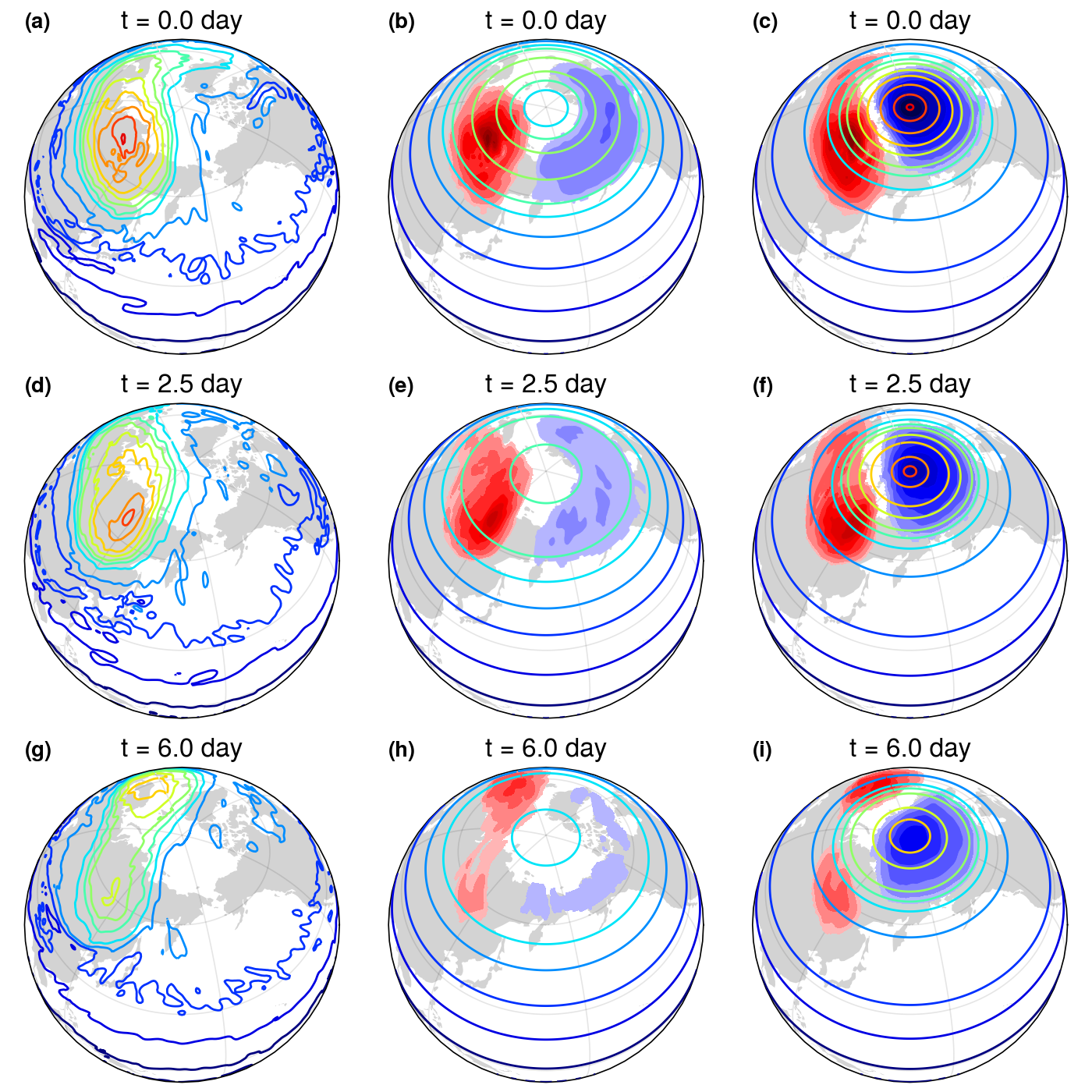
Here it is demonstrated that different eddy-mean flow decompositions. Eddies relative to zonal-mean state are weaker and near wavenumber-1 asymmetric about the pole. The ones relative to the reference state is much persistent and no clear WN-1 asymmetricity.
References
Nakamura, N., and A. Solomon, 2011: Finite-amplitude wave activity and mean flow adjustments in the atmospheric general circulation. Part II: Analysis in the isentropic coordinate. J. Atmos. Sci., 68, 2783-2799.
Thuburn, J., and V. Lagneau, 1999: Eulerian mean, contour integral, and finite-amplitude wave activity diagnostics applied to a single-layer model of the winter stratosphere. J. Atmos. Sci., 56, 689-710.