Bretherton steady flow over topography

01 May 2023 by MiniUFO

---

[TOC]

---

1. Introduction

It is well known that 2D inviscid and adiabatic shallow-water flows in terms of PV \(q\):

\[\begin{align} \frac{d q}{d t}&=\frac{d}{dt} \left(\frac{\zeta+f}{\eta-\eta_B}\right)=\frac{d}{dt}\left( \frac{\zeta+f}{h}\right) =0\tag{1} \end{align}\]

have two global invariants: total (kinetic) energy \(E=\int h(u^2+v^2)/2 dA\) and total enstrophy \(Q=\int h q^2/2dA\). Here \(h=\eta-\eta_B\) is the fluid thickness. Bretherton and Haidvogel (1976) have shown that, under QG approximation, if the flow is initially given an energy \(E_0\) over topography \(\eta_B\), then an steady-state flow can be obtained by minimizing the enstrophy \(Q\). At the same year, Salman et al. (1976) also derived the same model but from a perspective of statistical mechanics. Here we are going to reproduced their steady state solution using xinvert.

2. Derivation through a variational principle

Under the QG approximations, PV can be expressed as:

\[\begin{split}\begin{align} q&\approx\frac{\zeta_g+f_0+\beta y}{D-\eta_B}\notag\\ &\approx\frac{1}{D}\left(\zeta_g+f_0+\beta y+\frac{f_0}{D}\eta_B\right)\notag\\ &=\frac{1}{D}\left(\nabla^2\psi+f_0+\beta y+\frac{f_0}{D}\eta_B\right)\tag{2} \end{align}\end{split}\]

The second approximation is made if the variation of topography \(\eta_B\) is small compared to the constant total depth \(D\), that is \(\eta_B\ll D\). According to Bretherton and Haidvogel (1976), minimizing enstrophy with an initial total energy \(E_0\) is equivalent to a variational problem of the functional:

\[\begin{align} J[\psi]=Q[\psi]+\lambda (E[\psi] - E_0) \tag{3} \end{align}\]

where \(\lambda\) is the Lagrangian multiplier. The stationary point is obtained by taking the first variation as:

\[\begin{align} \delta J=\delta Q+\lambda \delta E = 0 \tag{4} \end{align}\]

where:

\[\begin{split}\begin{align} \delta Q&=\delta\int D\frac{1}{2}q^2 dA=\int Dq\delta q dA\notag\\ &=\int \frac{1}{D}\left(\nabla^2\psi+f_0+\beta y+\frac{f_0}{D}\eta_B\right)\delta \nabla^2\psi dA\notag\\ &=\int \frac{1}{D}\nabla^2\left(\nabla^2\psi+\frac{f_0}{D}\eta_B\right) \delta\psi dA = 0\tag{5}\\ \notag\\ \delta E &=\delta\int D\frac{1}{2}\left(\nabla\psi\right)^2dA\notag\\ &=\int D\nabla\psi\delta\left(\nabla\psi\right) dA =\int -D\nabla^2\psi\delta\psi dA \tag{6}W \end{align}\end{split}\]

Substitute Eqs. (5-6) into Eq. (4), one gets:

\[\begin{align} \delta J &=\int \left[ \frac{1}{D}\nabla^2\left(\nabla^2\psi+\frac{f_0}{D}\eta_B-\lambda D \psi\right)\right]\delta\psi dA = 0 \tag{7} \end{align}\]

For arbitary variations of \(\delta \psi\), only when:

\[\begin{align} \nabla^2\psi - \lambda D\psi = -\frac{f_0}{D}\eta_B \tag{8} \end{align}\]

is satisfied does the steady-state flow \(\psi_s\) can be found. In this case, Eq. (8) is an elliptical equation about \(\psi\) when topography \(\eta_B\) is prescribed (also other constant parameters). \(\lambda\) is determined by the initial energy \(E_0\) as:

\[\begin{align} E_0 = \int D \left(\nabla \psi_s\right)^2 dA \tag{9} \end{align}\]

It is NOT trivial to express \(\lambda\) in terms of \(E_0\), but the pattern of \(\psi_s\) does not change with different \(E_0\) or \(\lambda\) (only magnitude does).

3. Examples

Here we will demonstrate how to use xinvert python package to invert the 2D steady-state flow over topography undef QG case. First, we generate a random topography over a rectanglar domain.

import numpy as np
import xarray as xr

def add_bump(topo):
    num = 50
    xpos = np.random.rand(num) * topo.x.max().values * 0.8 + 15000
    ypos = np.random.rand(num) * topo.y.max().values * 0.8 + 10000
    rads = np.random.rand(num) * 9e9 + 8e9
    amps = np.random.rand(num) - 0.5

    bumps = sum(amp * np.exp(-((ydef-yo)**2 + (xdef-xo)**2)/rad) for amp, xo, yo, rad in zip(amps, xpos, ypos, rads))

    return topo.rename('topo') + bumps

xdef = xr.DataArray(np.linspace(0, 1500000, 301), dims='x', coords={'x':np.linspace(0, 1500000, 301)})
ydef = xr.DataArray(np.linspace(0, 1000000, 201), dims='y', coords={'y':np.linspace(0, 1000000, 201)})

# it is random topography, different from every run! So store it.
# topo.to_netcdf('../../../Data/topo.nc')

### classical cases ###
import sys
sys.path.append('../../../')
import numpy as np
import xarray as xr
from xinvert import invert_BrethertonHaidvogel, cal_flow

iParams = {
    'BCs'      : ['fixed', 'fixed'],
    'mxLoop'   : 3000,
    'tolerance': 1e-16,
    'undef'    : np.nan}

topo = xr.open_dataset('../../../Data/topo.nc').topo

mParams1 = {'f0': 1e-4, 'D': 1000, 'lambda': 1e-14}
mParams2 = {'f0': 1e-4, 'D': 1000, 'lambda': 3e-14}
mParams3 = {'f0': 1e-4, 'D': 1000, 'lambda': 1e-13}
mParams4 = {'f0': 1e-4, 'D': 1000, 'lambda': 3e-13}

S1 = invert_BrethertonHaidvogel(topo, dims=['y','x'], coords='cartesian', mParams=mParams1, iParams=iParams)
S2 = invert_BrethertonHaidvogel(topo, dims=['y','x'], coords='cartesian', mParams=mParams2, iParams=iParams)
S3 = invert_BrethertonHaidvogel(topo, dims=['y','x'], coords='cartesian', mParams=mParams3, iParams=iParams)
S4 = invert_BrethertonHaidvogel(topo, dims=['y','x'], coords='cartesian', mParams=mParams4, iParams=iParams)

u1, v1 = cal_flow(S1, dims=['y','x'], coords='cartesian')
u2, v2 = cal_flow(S2, dims=['y','x'], coords='cartesian')
u3, v3 = cal_flow(S3, dims=['y','x'], coords='cartesian')
u4, v4 = cal_flow(S4, dims=['y','x'], coords='cartesian')

E1 = (u1**2 + v1**2).sum() / 2
E2 = (u2**2 + v2**2).sum() / 2
E3 = (u3**2 + v3**2).sum() / 2
E4 = (u4**2 + v4**2).sum() / 2

{} loops 1136 and tolerance is 0.000000e+00
{} loops 1157 and tolerance is 0.000000e+00
{} loops 1133 and tolerance is 0.000000e+00
{} loops 1116 and tolerance is 0.000000e+00

Here we choose four sets of parameters for the inversion, and to see how the steady state flows depends on these parameters.

import proplot as pplt

skip = 5
fontsize = 11
ygrid, xgrid = xr.broadcast(topo.y, topo.x)

def plot_panel(ax, S, u, v, title, E):
    ax.contour(S, levels=11, color='k', lw=0.8)
    ax.contour(S, levels=[0], color='k', lw=2)
    m = ax.contourf(topo, levels=np.linspace(-0.8, 0.8, 20), cmap='bwr')
    ax.quiver(xgrid.values[::skip+1,::skip], ygrid.values[::skip+1,::skip],
              u.values[::skip+1,::skip], v.values[::skip+1,::skip],
              width=0.0014, headwidth=8., headlength=12., scale=50)
    ax.set_ylabel('y-coordinate (km)', fontsize=fontsize-1)
    ax.set_xlabel('x-coordinate (km)', fontsize=fontsize-1)
    ax.set_yticks([0, 2e5, 4e5, 6e5, 8e5, 1e6])
    ax.set_xticks([0, 3e5, 6e5, 9e5, 1.2e6, 1.5e6])
    ax.set_yticklabels(['0', '200', '400', '600', '800', '1000'])
    ax.set_xticklabels(['0', '300', '600', '900', '1200', '1500'])
    ax.set_title(title + ',  total KE: {:6.5f}'.format(E), fontsize=fontsize)

    return m

fig, axes = pplt.subplots(nrows=2, ncols=2, figsize=(7,5), sharex=3, sharey=3)

m = plot_panel(axes[0,0], S1, u1, v1, '$\\lambda=1E-14$', E1.values)
m = plot_panel(axes[0,1], S2, u2, v2, '$\\lambda=3E-14$', E2.values)
m = plot_panel(axes[1,0], S3, u3, v3, '$\\lambda=1E-13$', E3.values)
m = plot_panel(axes[1,1], S4, u4, v4, '$\\lambda=3E-13$', E4.values)

fig.colorbar(m, loc='b', label='topography', ticks=0.1, cols=(1,2))
axes.format(abc='(a)')

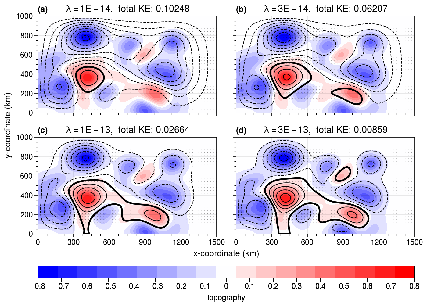
In the above plot, we show the topography (shaded) and streamfunction (contours), with flow vector superimposed. It is clear that if the initial total KE is large, then \(\lambda\) should be small. The larger KE, the smoother the streamfunction. This is in accordance with Bretherton and Haidvogel (1976). They also noted that it is not easy to get an explicit expression between \(\lambda\) and \(E_0\). We can try their relation with many runs here.

lambdas = np.linspace(1e-15, 1e-12, 50)

Es = []

iParams['printInfo'] = False

for i, lm in enumerate(lambdas):
    if i % 10 == 0:
        print(i, '   ', lm)
    mParams = {'f0': 1e-4, 'D': 1000, 'lambda': lm}
    S1 = invert_BrethertonHaidvogel(topo, dims=['y','x'], coords='cartesian', mParams=mParams, iParams=iParams)
    u1, v1 = cal_flow(S1, dims=['y','x'], coords='cartesian')
    Es.append((u1**2 + v1**2).sum() / 2)

Es = np.array(Es)

0     1e-15
10     2.0487755102040815e-13
20     4.087551020408163e-13
30     6.126326530612244e-13
40     8.165102040816326e-13

import proplot as pplt

fig, axes = pplt.subplots(nrows=2, ncols=2, figsize=(7,5), sharex=0, sharey=0)

fontsize = 12

ax = axes[0, 0]
ax.scatter(lambdas, Es)
ax.set_ylabel('$E_K$', fontsize=fontsize-1)
ax.set_xlabel('$\\lambda$', fontsize=fontsize-1)
ax.set_title('$\\lambda$ vs $E_K$ (original)', fontsize=fontsize-1)

ax = axes[0, 1]
ax.scatter(lambdas, Es)
ax.set_xscale('log')
ax.set_xticks(np.array([0.001, 0.01, 0.1, 1])*1e-12)
ax.set_ylabel('$E_K$', fontsize=fontsize-1)
ax.set_xlabel('$\\lambda$', fontsize=fontsize-1)
ax.set_title('$\\lambda$ vs $E_K$ (log_x)', fontsize=fontsize-1)

ax = axes[1, 0]
ax.scatter(lambdas, Es)
ax.set_yscale('log')
ax.set_yticks([1e-3, 3e-3, 1e-2, 3e-2, 1e-1, 3e-1])
ax.set_ylabel('$E_K$', fontsize=fontsize-1)
ax.set_xlabel('$\\lambda$', fontsize=fontsize-1)
ax.set_title('$\\lambda$ vs $E_K$ (log_y)', fontsize=fontsize-1)

ax = axes[1, 1]
ax.scatter(lambdas, Es)
ax.set_yscale('log')
ax.set_xscale('log')
ax.set_xticks(np.array([0.001, 0.01, 0.1, 1])*1e-12)
ax.set_yticks([1e-3, 3e-3, 1e-2, 3e-2, 1e-1, 3e-1])
ax.set_ylabel('$E_K$)', fontsize=fontsize-1)
ax.set_xlabel('$\\lambda$', fontsize=fontsize-1)
ax.set_title('$\\lambda$ vs $E_K$ (log_xy)', fontsize=fontsize-1)

axes.format(abc='(a)')

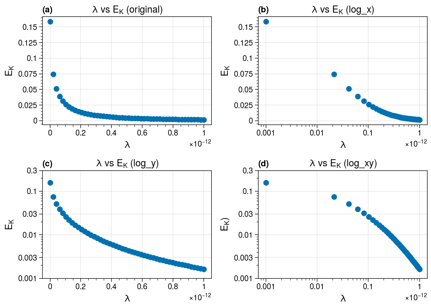
Well, it is clear that NO simple relation between \(K_E\) and \(\lambda\). Their relation also depends on the topography.

---

References

1. Bretherton, F. P., and D. Haidvogel, 1976: Two-dimensional turbulence above topography. J. Fluid Mech., 78, 129-154.

2. Salmon, R., G. Holloway, and M. Hendershott, 1976: The equilibrium statistical mechanics of simple quasi-geostrophic models. J. Fluid Mech., 75, 691-703.